Tutorial 1 - A Quick Demo

In this first tutorial, we want to present some basics of DASF framework and how you can use it to manage your machine learning algorithms in a multi architecture environemnt like single machines, clusteres and GPUs.

If you are familiar with all the scikit-learn API, DASF has the same methodology of function notations. The only difference of DASF is that this framework is directly associated with the host environment. If you are using a clustered environment with Dask for example, you will use the optimized functions for that environment type. If you are running your code in a single GPU host environment, your code will have the specific optimizations for that type and so on so forth.

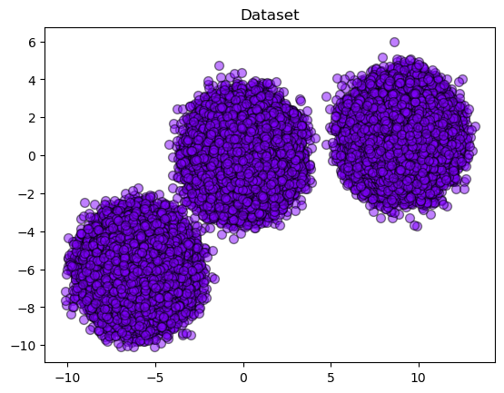
Let’s try our first example with some basic clustering algorithm. First, create a simple dataset using make_blobs function.

from dasf.datasets import make_blobs

n_samples = 500000
n_bins = 3

# Generate 3 blobs with 2 classes where the second blob contains
# half positive samples and half negative samples. Probability in this
# blob is therefore 0.5.
centers = [(-6, -6), (0, 0), (9, 1)]
X, y = make_blobs(n_samples=n_samples, centers=centers, shuffle=False, random_state=42)

Notice that we are using the same code available in scikit-learn tutorials and demos.

To have a better view of the data distribution, we can plot the generated dataset.

# Only to generate colors
import numpy as np

from dasf.utils.types import is_gpu_array

from matplotlib import cm
import matplotlib.pyplot as plt

# Check the data just to plot
if is_gpu_array(X):
    X_cpu = X.get()
else:
    X_cpu = X

colors = cm.rainbow(np.linspace(0.0, 1.0, 1))

plt.figure()
plt.scatter(
    X_cpu[:, 0],
    X_cpu[:, 1],
    s=50,
    c=colors[np.newaxis, :],
    alpha=0.5,
    edgecolor="k",
)
plt.title("Dataset")

plt.show()

Once, we have the big picture of how our dataset is distributed, let’s run two clustering algorithms to understand how it can be classified.

For this tutorial, we decided to use KMeans and SOM (Kohonen’s Self-Organized Map) as an example.

from dasf.ml.cluster import KMeans
from dasf.ml.cluster import SOM

kmeans = KMeans(n_clusters=3, max_iter=100)
som = SOM(x=1, y=3, input_len=2, num_epochs=100)

As we know our dataset defines 3 centers with 2 classes, we set KMeans n_clusters parameter with the same number of classes of our dataset. On the other hand, SOM is based on an activation map and it does not necessary needs a 1-D map with 3 activation points, but we want to use here to help the classification algorithm also. See that as we also know that our dataset contains two classes, the parameter input_len of SOM needs to be set as 2 (same number of classes).

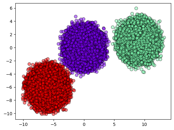
Now, it is time to fit_predict both classifiers. Let’s analyze KMeans first.

%time result_kmeans = kmeans.fit_predict(X)

CPU times: user 315 ms, sys: 7.29 ms, total: 322 ms
Wall time: 326 ms

KMeans is a fast algorithm compared to SOM. For further reference, let’s see the speed of the SOM algorithm.

%time result_som = som.fit_predict(X)

CPU times: user 4min, sys: 210 ms, total: 4min
Wall time: 4min 1s

Now, let’s see the performance of each prediction. The first one is KMeans results.

from itertools import cycle

def plot_results(X, result):
    y_unique = np.unique(result)

    colors = cm.rainbow(np.linspace(0.0, 1.0, y_unique.size))

    for this_y, color in zip(y_unique, colors):
        if is_gpu_array(X):
            this_X = X[result == this_y].get()
        else:
            this_X = X[result == this_y]

        plt.scatter(
            this_X[:, 0],
            this_X[:, 1],
            s=50,
            c=color[np.newaxis, :],
            alpha=0.5,
            edgecolor="k",
            label="Class %s" % this_y,
        )

plot_results(X, result_kmeans)

Now, let’s see how SOM results look like.

plot_results(X, result_som)

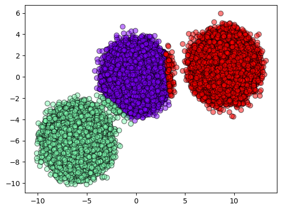
As we can see, the results do not seem similar but they are accurated.

The idea behind this tutorial is not to exaplain how both algorithms work, but how can you use DASF framework the same way you use the most famous Machine Learning libraries.

If you are curious, try to run the same code using a machine with GPU. Compare the results and see if the behaviour is the same!