Tutorial 4 - How Create an Agnostic Pipeline

In this tutorial, we will show you how convert a simple code structure into a advanced and agnostic pipeline based on DAGs.

For this, we still can use the Tutorial 1 with a simple Machine Learning script. There we use make_blobs to generate a dataset and them we cluster it using two algorithms: KMeans and SOM.

First, let’s generate and save our data (you can use DASF or Scikit-learn). The objective here is just to generate some labeled data and use the DatasetLabeled as an example.

import numpy as np

from dasf.datasets import make_blobs

n_samples = 100000
n_bins = 3

# Generate 3 blobs with 2 classes where the second blob contains
# half positive samples and half negative samples. Probability in this
# blob is therefore 0.5.
centers = [(-6, -6), (0, 0), (9, 1)]
X, y = make_blobs(n_samples=n_samples, centers=centers, shuffle=False, random_state=42)

np.save("X.npy", X)
np.save("y.npy", y)

Now, let’s import our DatasetLabeled and assign each file to the respective type.

from dasf.datasets import DatasetArray
from dasf.datasets import DatasetLabeled


class MyMakeBlobs(DatasetLabeled):
    def __init__(self):
        super().__init__(name="My Own make_blobs()", download=False)

        # Let's assign the train and val data.
        self._train = DatasetArray(name="X", download=False, root="X.npy", chunks=(5000, 2))
        self._val = DatasetArray(name="y", download=False, root="y.npy", chunks=(5000))

make_blobs = MyMakeBlobs()

To reduce the variability and as an example, we can normalize the data to help the algorithms to fit better.

from dasf.transforms import Normalize

normalize = Normalize()

After, creating our dataset and the normalization transformation, we can start the executor. For this example, we can use Dask.

from dasf.pipeline.executors import DaskPipelineExecutor

dask = DaskPipelineExecutor(local=True, use_gpu=False)

Now, it is time to create our pipeline objects. We can copy and paste the same code used previously.

from dasf.ml.cluster import KMeans
from dasf.ml.cluster import SOM

kmeans = KMeans(n_clusters=3, max_iter=100)
som = SOM(x=1, y=3, input_len=2, num_epochs=100)

WARNING: CuPy could not be imported
WARNING: CuPy could not be imported
WARNING: CuPy could not be imported

As we want to reuse the data after the pipeline execution, we need to persist the data.

from dasf.transforms import PersistDaskData

persist_kmeans = PersistDaskData()
persist_som = PersistDaskData()

Then, we generate the pipeline and connect all the pieces in one single DAG.

Pay attention that we are passing the our fresh executor dask to the pipeline by specifying the parameter executor=.

To connect all the objects, we use the function add() that returns the pipeline itself. The function inputs can be refered as an argument.

At the end, we can visualize the DAG using visualize() method. It will plot a image that represents the graph. Let’s use one single line to do everything. It should be simple and easy to understand.

from dasf.pipeline import Pipeline

pipeline = Pipeline("A KMeans and SOM Pipeline", executor=dask)

pipeline.add(normalize, X=make_blobs._train) \
        .add(kmeans.fit_predict, X=normalize) \
        .add(som.fit_predict, X=normalize) \
        .add(persist_kmeans, X=kmeans.fit_predict) \
        .add(persist_som, X=som.fit_predict) \
        .visualize()

It is time to run our new pipeline.

%time pipeline.run()

[2022-11-25 04:36:49+0000] INFO - Beginning pipeline run for 'A KMeans and SOM Pipeline'
[2022-11-25 04:36:49+0000] INFO - Task 'DatasetArray.load': Starting task run...
[2022-11-25 04:36:50+0000] INFO - Task 'DatasetArray.load': Finished task run
[2022-11-25 04:36:50+0000] INFO - Task 'Normalize.transform': Starting task run...
[2022-11-25 04:36:50+0000] INFO - Task 'Normalize.transform': Finished task run
[2022-11-25 04:36:50+0000] INFO - Task 'KMeans.fit_predict': Starting task run...

/usr/local/lib/python3.8/dist-packages/dask/base.py:1367: UserWarning: Running on a single-machine scheduler when a distributed client is active might lead to unexpected results.
  warnings.warn(

[2022-11-25 04:37:00+0000] INFO - Task 'KMeans.fit_predict': Finished task run
[2022-11-25 04:37:00+0000] INFO - Task 'SOM.fit_predict': Starting task run...
[2022-11-25 04:37:22+0000] INFO - Task 'SOM.fit_predict': Finished task run
[2022-11-25 04:37:22+0000] INFO - Task 'PersistDaskData.transform': Starting task run...
[2022-11-25 04:37:22+0000] INFO - Task 'PersistDaskData.transform': Finished task run
[2022-11-25 04:37:22+0000] INFO - Task 'PersistDaskData.transform': Starting task run...
[2022-11-25 04:37:23+0000] INFO - Task 'PersistDaskData.transform': Finished task run
[2022-11-25 04:37:23+0000] INFO - Pipeline run successfully
CPU times: user 23.2 s, sys: 1.71 s, total: 24.9 s
Wall time: 33.2 s

Notice that our pipeline returns two methods instead of one. To capture the result of some node, you can easily pass the same function or object to the pipeline function get_result_from().

result_kmeans = pipeline.get_result_from(persist_kmeans).compute()
result_som = pipeline.get_result_from(persist_som).compute()

import numpy as np

from itertools import cycle

from matplotlib import cm
import matplotlib.pyplot as plt

def plot_results(X, result):
    y_unique = np.unique(result)

    colors = cm.rainbow(np.linspace(0.0, 1.0, y_unique.size))

    for this_y, color in zip(y_unique, colors):
        this_X = X[result == this_y]
        plt.scatter(
            this_X[:, 0],
            this_X[:, 1],
            s=50,
            c=color[np.newaxis, :],
            alpha=0.5,
            edgecolor="k",
            label="Class %s" % this_y,
        )

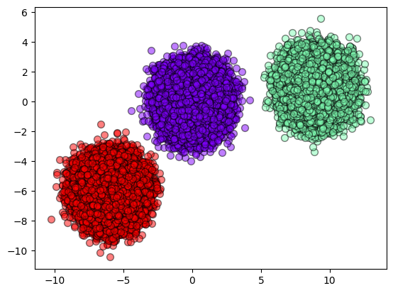
plot_results(make_blobs._train, result_kmeans)

plot_results(make_blobs._train, result_som)